Theory

The original Phong lighting model classifies the light coming into the eye into four distinct categories. A diffuse contribution that represents light shattered in every direction evenly. A specular contribution that represents light reflected mostly in a perfect mirror bounce. An ambient contribution to account for all indirect light that it scattered around the scene. And finally an emissive contribution for the light that is being emitted from the surface itself. The emissive contribution is a special case for surfaces that emit light, such as the surface of a lightbulb or the sun. We don’t have any light emitting surfaces in our example program so we won’t be discussing it any further.

Blinn’s modification to the Phong shading model is in the way the specular contribution is computed. But before we get to that lets first look at how to compute the other two contributions.

The ambient contribution is the easiest of the three to compute. It is used to account for light that bounces more than one time before it enters the eye, so called ambient light. To compute it we simply multiply the global ambient value with the ambient value of the surface we wish to shade.

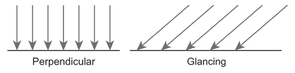
The diffuse contribution represents light that travels directly from the light source to the shading point and is shattered in all directions evenly due to the rough nature of the surface material. When computing this contribution we have to take into account Lambert’s Law, which states that surfaces perpendicular to rays of light receive more light per unit area than surfaces at a more glancing angle.

To compute the diffuse contribution we first multiply the diffuse component of the light with the diffuse component of the object. To account for Lambert’s Law we multiply this value with the cosine of the angle between the direction of the light and the normal of the surface we are shading. We become the cosine by taking the dot product of the light direction vector and the surface normal.

Likewise to the diffuse contribution, the specular component represents light that travels directly from the light source to the shading point. Different from the diffuse component, the specular contribution represents light that is reflected mostly in a perfect mirror bounce, it’s what gives surfaces a shiny appearance. In the Phong lighting model the specular contribution is computed by taking the cosine of the angle between the reflectance vector and the view direction vector. Which we once again become by taking the dot product of these two vectors.

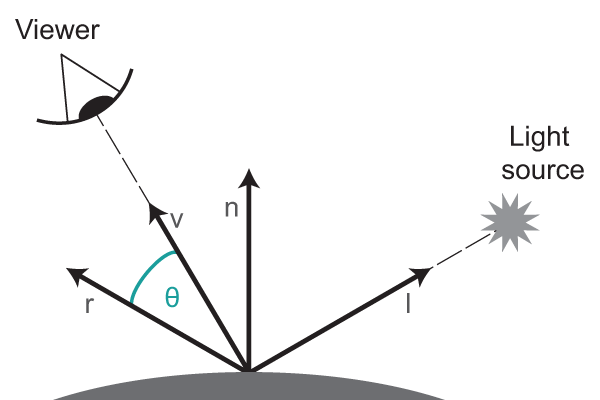
The result of the dot product is taken to the power of the material shininess value, this specifies how big or small the hotspot around the reflectance vector is, a smaller shininess value produces a larger hotspot and a larger value produces a smaller sharper hotspot. Finally the resulting value is multiplied with the product of the specular value of the light and the surface material.

Blinn’s modification is an optimization for the way the specular contribution is computed. Instead of using the cosine of the angle between the reflectance and view direction vectors, Blinn proposes to use the cosine value between the halfway vector and the surface normal. The halfway vector is the average of the view direction vector and the light direction vector. This way we avoid computing the reflectance vector. Another optimization that Blinn introduced is that we can treat the view direction as a constant for objects that are far away from the viewer. Likewise we can treat the light direction vector as a constant for objects that are far away from the light source. If both the viewer and the light source are far away from the object we only have to compute the halfway vector once for the entire object and the given light source.

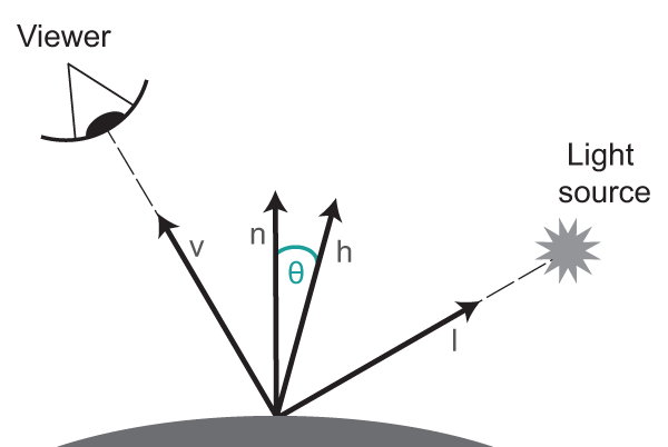
Blinn’s formula for specular reflection is very similar to Phong’s formula, only the factors of the dot product are changed.

Finally we become the light value by adding up all contributions.

Implementation

Now that we covered the basics of the Blinn-Phong lighting model we can move on to the implementation. We start by defining the location and lighting properties of our light source, which is a point light in our case.

...

var lightPosition = vec4(-1.5, 2.0, 4.0, 1.0);
var lightAmbient = vec4(0.2, 0.2, 0.2, 1.0);
var lightDiffuse = vec4(1.0, 1.0, 1.0, 1.0);
var lightSpecular = vec4(1.0, 1.0, 1.0, 1.0);

...
}

Next we define the material of our cube object. Similar to the light source we must define an ambient, diffuse and specular component. We have to define one more lighting property for the material and that’s the shininess value. This value is used to compute the specular value and defines how fast the specular reflection drops off. How higher the shininess value how smaller and more focused the specular reflection area will be.

window.onload = function init()
{
  ...

  var materialAmbient = vec4(0.0, 1.0, 0.0, 1.0);
  var materialDiffuse = vec4(0.4, 0.8, 0.4, 1.0);
  var materialSpecular = vec4(0.0, 0.4, 0.4, 1.0);
  var materialShininess = 300.0;

  ...
}

To shade our object we’ll also need the surface normals. In each execution of the vertex shader we can only access one vertex element. However to compute the normals for a triangular face we need all three vertices. This means we need to compute the normals in the application program and send them to the vertex shader. In our example project we fill the normals array by passing it as an argument to the faces_as_triangles function. For more info on how this function works and how the surface normals are computed you can download the source files of this project and take a look yourself.

window.onload = function init()
{
  ...

  var points = [];
  var normals = [];
  points = points.concat(cube.faces_as_triangles(normals));

  ...
}

We transfer the normals array to the shaders the same way we transferred the points array in the original rotating cube project.

window.onload = function init()
{
  ...

  var nBuffer = gl.createBuffer();
  gl.bindBuffer(gl.ARRAY_BUFFER, nBuffer);
  gl.bufferData(gl.ARRAY_BUFFER, flatten(normals), gl.STATIC_DRAW);

  var vNormal = gl.getAttribLocation(program, "vNormal");
  gl.vertexAttribPointer(vNormal, 4, gl.FLOAT, false, 0, 0);
  gl.enableVertexAttribArray(vNormal);

  ...
}

We also need to pass the light and material properties to the shaders. For the ambient, diffuse and specular components we can compute the product of the light and material values in the application program, this way we have to transfer less data between the CPU and the GPU and we avoid computing the product every time the shader is executed.

window.onload = function init()
{
  ...

  var lightPositionLoc =
    gl.getUniformLocation(program, "lightPosition");
  gl.uniform4fv(lightPositionLoc, flatten(lightPosition));

  var ambientProduct = mult(lightAmbient, materialAmbient);
  var ambientProductLoc =
    gl.getUniformLocation(program, "ambientProduct");
  gl.uniform4fv(ambientProductLoc, flatten(ambientProduct));

  var diffuseProduct = mult(lightDiffuse, materialDiffuse);
  var diffuseProductLoc =
    gl.getUniformLocation(program, "diffuseProduct");
  gl.uniform4fv(diffuseProductLoc, flatten(diffuseProduct));

  var specularProduct = mult(lightSpecular, materialSpecular);
  var specularProductLoc =
    gl.getUniformLocation(program, "specularProduct");
  gl.uniform4fv(specularProductLoc, flatten(specularProduct));

  var shininessLoc = gl.getUniformLocation(program, "shininess");
  gl.uniform1f(shininessLoc, materialShininess);


  ...
}

Now that we have everything set up we can move on to our shaders where the actual lighting computation will happen. The first thing we do in the vertex shader, similar to the original rotating cube shader, is computing the rotation matrices for the rotation.

<script id="vertex-shader" type="x-shader/x-vertex">
  uniform vec3 theta;

  void main()
  {
    vec3 angles = radians(theta);
    vec3 c = cos(angles);
    vec3 s = sin(angles);
    mat4 rx = mat4(
      1.0, 0.0, 0.0, 0.0,
      0.0, c.x, s.x, 0.0,
      0.0, -s.x, c.x, 0.0,
      0.0, 0.0, 0.0, 1.0
    );
    mat4 ry = mat4(
      c.y, 0.0, -s.y, 0.0,
      0.0, 1.0, 0.0, 0.0,
      s.y, 0.0, c.y, 0.0,
      0.0, 0.0, 0.0, 1.0
    );

    ...
  }
</script>

First we apply this rotation to the vertex position. Because we will do the lighting computation in view/camera space we also apply the model-view matrix to both the vertex position and the light position.

<script id="vertex-shader" type="x-shader/x-vertex">
  attribute vec4 vPosition;

  uniform mat4 modelViewMatrix;
  uniform vec4 lightPosition;

  void main()
  {
    ...

    vec3 pos = (modelViewMatrix * rx * ry * vPosition).xyz;
    vec3 lightPos = (modelViewMatrix * lightPosition).xyz;

    ...
  }
</script>

Next we become the light direction vector, by subtracting the light position vector from the vertex position and normalizing the result.

<script id="vertex-shader" type="x-shader/x-vertex">
  void main()
  {
    ...

    L = normalize(lightPos - pos);

    ...
  }
</script>

We also need to apply the rotation and the model-view transform to the vertex normal. Keep in mind that in general normals must be transformed with the inverse transpose of the transformation matrix. But because our transformation does not contain non-uniform scale we can safely ignore this fact. All we need to do is renormalize the normal after the transformation.

<script id="vertex-shader" type="x-shader/x-vertex">
  attribute vec4 vNormal;

  void main()
  {
    ...

    N = normalize((modelViewMatrix * rx * ry * vNormal).xyz);

    ...
  }
</script>

Finally we also need to define the view/eye direction vector. We are doing the shading in view space, this means the camera is positioned at the origin or the coordinate system. So to get the view direction vector we simply negate and normalize the transformed vertex position.

<script id="vertex-shader" type="x-shader/x-vertex">
  void main()
  {
    ...

    E = -normalize(pos);

    ...
  }
</script>

The full vertex shader is shown below. Notice that at the end of the shader we apply the rotation, model-view transform and projection transform to the vertex coordinates, just as we did in the original rotating cube program.

<script id="vertex-shader" type="x-shader/x-vertex">
  attribute vec4 vNormal;
  attribute vec4 vPosition;
  varying vec3 L, N, E;

  uniform mat4 modelViewMatrix;
  uniform mat4 projectionMatrix;
  uniform vec3 theta;
  uniform vec4 lightPosition;

  void main()
  {
    vec3 angles = radians(theta);
    vec3 c = cos(angles);
    vec3 s = sin(angles);
    mat4 rx = mat4(
      1.0, 0.0, 0.0, 0.0,
      0.0, c.x, s.x, 0.0,
      0.0, -s.x, c.x, 0.0,
      0.0, 0.0, 0.0, 1.0
    );
    mat4 ry = mat4(
      c.y, 0.0, -s.y, 0.0,
      0.0, 1.0, 0.0, 0.0,
      s.y, 0.0, c.y, 0.0,
      0.0, 0.0, 0.0, 1.0
    );

    vec3 pos = (modelViewMatrix * rx * ry * vPosition).xyz;
    vec3 lightPos = (modelViewMatrix * lightPosition).xyz;

    L = normalize(lightPos - pos);
    N = normalize((modelViewMatrix * rx * ry * vNormal).xyz);
    E = -normalize(pos);

    gl_Position =
      projectionMatrix * modelViewMatrix * rx * ry * vPosition;
  }
</script>

We can now apply the Blinn-Phong lighting model to each fragment by using the ambient, diffuse and specular products passed in from the application and the interpolated light direction, normal and view direction vectors from the rasterizer.

For the diffuse value we start by taking the dot product of the light direction and the surface normal. We clamp the result to zero because the result of the dot product can be negative, in which case the light is behind the surface which the fragment is a part of. Finally we multiply the clamped dot product with the diffuse product passed in from the application to become the diffuse value for the fragment.

<script id="fragment-shader" type="x-shader/x-fragment">
  precision mediump float;
  varying vec3 L, N, E;

  uniform vec4 diffuseProduct;

  void main()
  {
    vec4 diffuse = max(dot(L, N), 0.0) * diffuseProduct;

    ...
  }
</script>

For the specular value we first need to compute the halfway vector, which we become by normalizing the sum of the light direction and view direction vectors. Next we take the dot product of the surface normal and the halfway vector, making sure to clamp the result to zero. We need to take the clamped dot product to the power of the shininess factor and then we can multiply it with the specular product to become the specular value for the fragment.

<script id="fragment-shader" type="x-shader/x-fragment">
  uniform vec4 specularProduct;
  uniform float shininess;

  void main()
  {
    ...

    vec3 H = normalize(L+E);
    vec4 specular =
      pow(max(dot(N, H), 0.0), shininess) * specularProduct;

    ...
  }
</script>

We have to do add more step for the specular value before we can move one. In case the dot product between the light direction and the surface normal is negative, which means the light is behind the surface, we want the specular value to be zero.

<script id="fragment-shader" type="x-shader/x-fragment">
  void main()
  {
    ...

    if (dot(L, N) < 0.0)
      specular = vec4(0.0, 0.0, 0.0, 1.0);

    ...
  }
</script>

We can now set the color of the value to the sum of the ambient, diffuse and specular lighting values. We set the alpha value of the color to 1.0 because we don’t want the material of the cube to be transparent.

<script id="fragment-shader" type="x-shader/x-fragment">
  uniform vec4 ambientProduct;

  void main()
  {
    ...

    vec4 fColor = ambientProduct + diffuse + specular;
    fColor.a = 1.0;

    gl_FragColor = fColor;
  }
</script>

The complete fragment shader:

<script id="fragment-shader" type="x-shader/x-fragment">
  precision mediump float;
  varying vec3 L, N, E;

  uniform vec4 ambientProduct;
  uniform vec4 diffuseProduct;
  uniform vec4 specularProduct;
  uniform float shininess;

  void main()
  {
    vec4 diffuse = max(dot(L, N), 0.0) * diffuseProduct;
    vec3 H = normalize(L+E);
    vec4 specular =
      pow(max(dot(N, H), 0.0), shininess) * specularProduct;

    if (dot(L, N) < 0.0)
      specular = vec4(0.0, 0.0, 0.0, 1.0);

    vec4 fColor = ambientProduct + diffuse + specular;
    fColor.a = 1.0;

    gl_FragColor = fColor;
  }
</script>

Use the download button to download the shaded rotating cube program. And if you have any questions or comments please leave a message below!